7 simple tips to clean up your datasets in Excel

Handling hundreds of rows, columns, and pivot tables usually results in a less-than-perfect dataset. A massive Excel workbook is often riddled with inconsistencies, errors, missing values, duplicates, and unnecessary formatting to derail your entire analysis. But this is where the power of Excel comes in. Microsoft’s spreadsheet solution offers a robust set of data-cleaning tools to transform chaotic data into a well-organized, analysis-ready foundation.

Whether you are a seasoned analyst or just starting your data journey, the tips below will help you conquer the art of data cleaning in Excel. It will surely squeeze out those annoying errors, streamline your workflow, and unlock the full potential of your data.

This is the first thing you need to do after creating a database in Excel. Although those extra spaces seem harmless, they are silent saboteurs, adding inconvenience in ways you might not even realize. These extra spaces distort your analysis, mess up sorting and filtering, and even cause mismatches and errors.

Use the Find and Replace tool

Find and Replace tool is one of the easiest ways to remove extra spaces in Excel. Let’s check it in action.

1. Open your Excel workbook.
2. Press the Ctrl + H (control + H on Mac) keys to open the Find and Replace dialog box.
3. In the Find What dialog box, press the space key twice.
4. Move to Replace With dialog box and press the space key once.
5. Click Replace All.

   

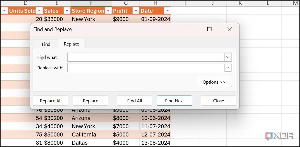
Excel should replace accidental double spaces with a single space.

If you don’t want to use the Find and Replace tool, explore the TRIM function in Excel to get the job done.

1. Create a new column next to the one with extra spaces. This will temporarily hold the cleaned data.
2. In the first cell of the new column, enter the TRIM formula. For example, if your original data is in column A and you’ve added a new column B, in cell B1, type =TRIM(A1).

   

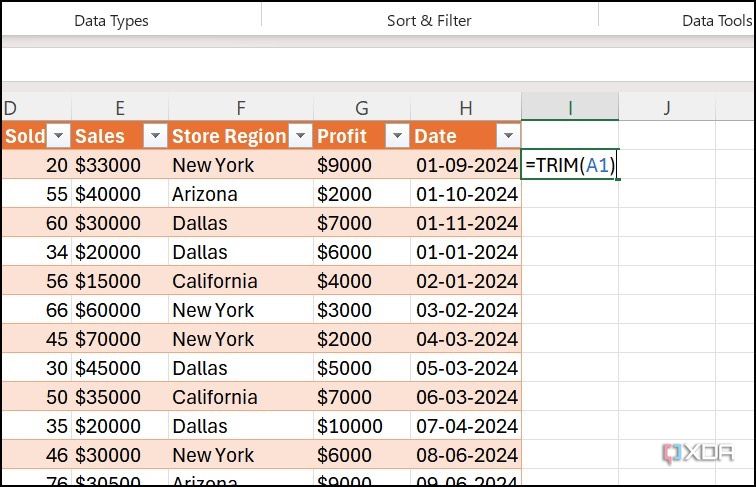
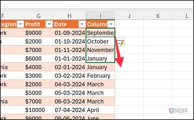
3. It displays the cleaned result in B1. Select the cell and move to the bottom right corner.
4. Click and drag the fill handle down the column until you reach the last row of your data. This will copy the TRIM formula to all the cells in column B.

   

5. Select all cells in the B column, and press Ctrl + C to copy the data.
6. Paste the same as values in the A column.

You can now delete the B column.

6 Remove all blank cells

Blank cells in Excel can be tricky. Sometimes, they are legitimate, throw errors, or just get in the way of your analysis. You can visually handle blank cells. But when you deal with large datasets, follow the steps below to handle them.

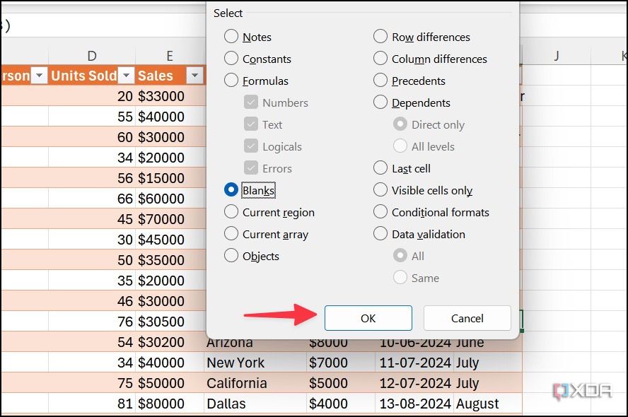
1. Open your Excel workbook and press the Ctrl + G keys to open the Go to dialog.
2. Click Special.

   

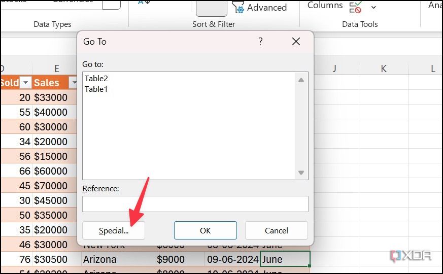
3. Select blank and click OK. It should highlight all the blank cells in your workbook.

   

Now, it’s up to you how to treat them. You can either remove entire rows or columns (with caution), replace them with specific values, fill with adjacent values (by dragging near cells), and more.

Related

12 Excel functions everyone should know about

Essential Microsoft Excel functions to streamline your everyday tasks

5 Run a spell check

Before you share your Excel workbook with others, make sure to run a spell check once to avoid any embarrassing errors.

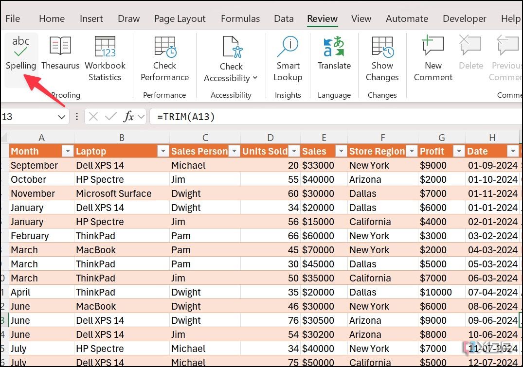
1. Open your Excel workbook and head to the Review tab at the top. Click Spelling.

   

2. Glance over suggestions and click Change or Ignore.

   

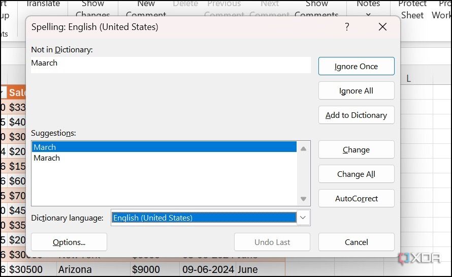
If you have a word that you use often but isn’t in Excel’s dictionary, click Add to Dictionary to prevent it from being flagged in the future.

4 Remove duplicates

This is another neat way to simplify your datasets in Microsoft Excel. The tool is built right into Excel.

1. Select Data on your Excel workbook.
2. Click Remove duplicates under Data Tools.

   

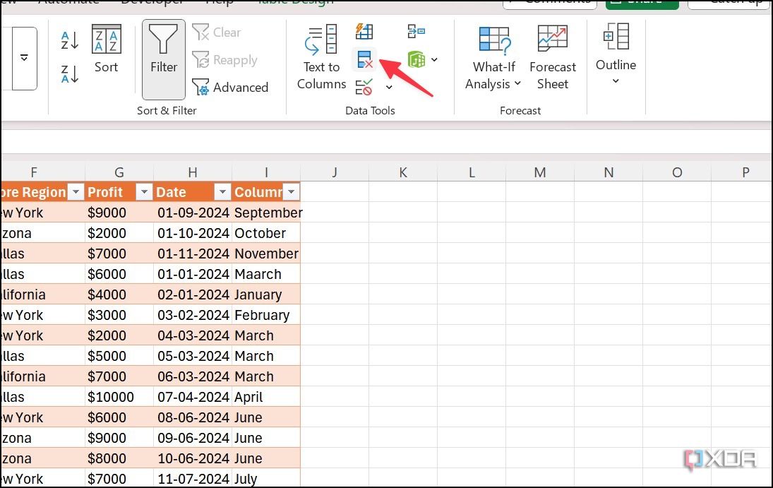
3. Select columns from which you want to remove duplicates. Click OK.

   

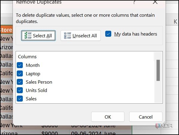
Excel displays a message showing the number of duplicate values removed.

Related

15 best Excel plugins that you need to be using

Must-have Excel add-ins you can’t afford to ignore

3 Clear formatting

In some cases, you may want to clear formatting from your Excel workbook. If it’s normal formatting like color, highlighter, or alignment, select cells, move to Home > Editing > Clear and select Clear formats.

If it’s conditional formatting, use the steps below.

1. Select Home > Conditional Formatting.
2. Expand Clear Rules and select Clear Rules from Entire Sheet or Selected Cells.

   

2 Change case

Do you want to manipulate data in an Excel sheet in terms of character cases? Use different functions to make changes.

• =UPPER(cell address) – Changes to upper case
• =LOWER(cell address) – Changes to lower case
• =PROPER(cell address) – For sentence case conversion

You can drag a cell and expand it to the bottom to apply the same across all the cells in the column.

Related

How to analyze data in Excel like a pro with pivot tables

Explore pivot tables to transform from a beginner to an analyst in minutes

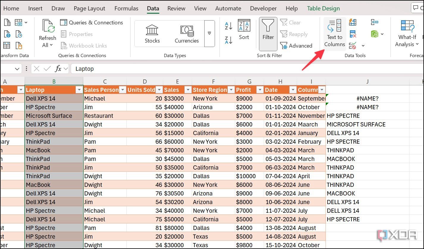
1 Data parsing from text to column

If your Excel workbook has customer information, device model number, address, and other information that’s separated by space, comma, or semicolon, you can clearly separate text in multiple columns.

1. Select a column from which you want to separate text.
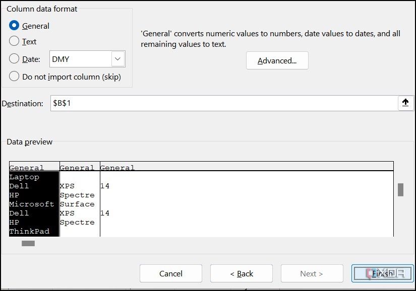
2. Select Data and open Convert Text to Columns Wizard.

   

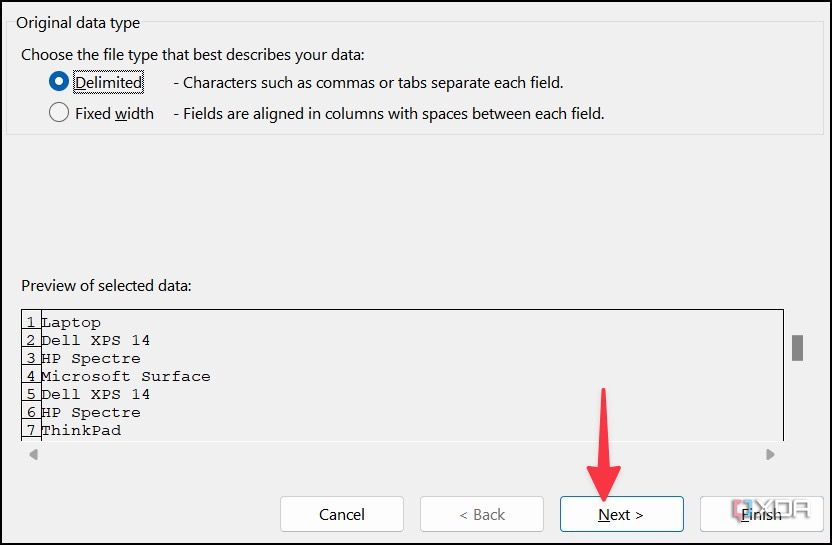
3. Glance over your column and select Next.

   

4. Select Tab, Semicolon, Command, Space, or other (specify by which you want to separate text).

   

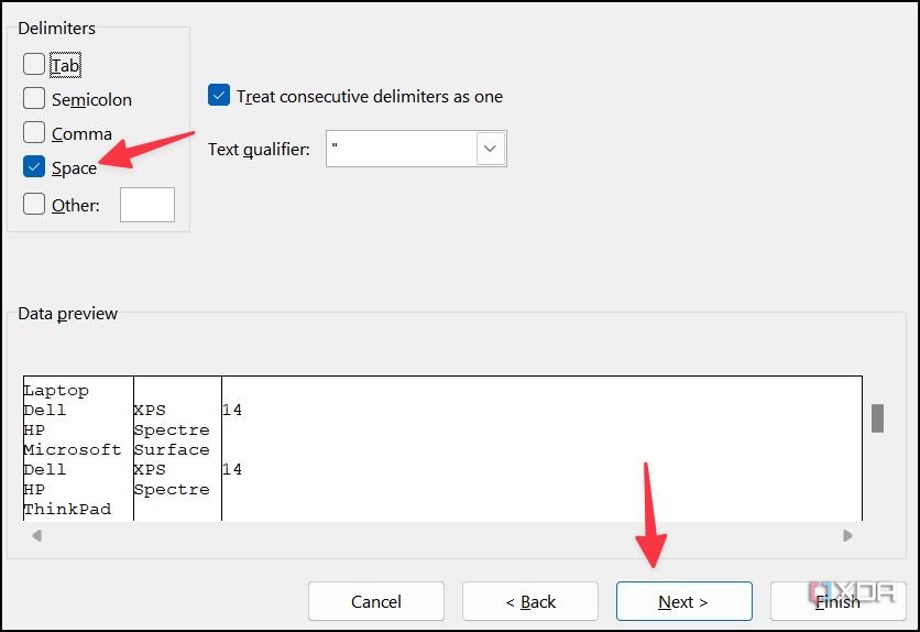
5. Click Next and glance over the preview with new columns. Select Finish.

   

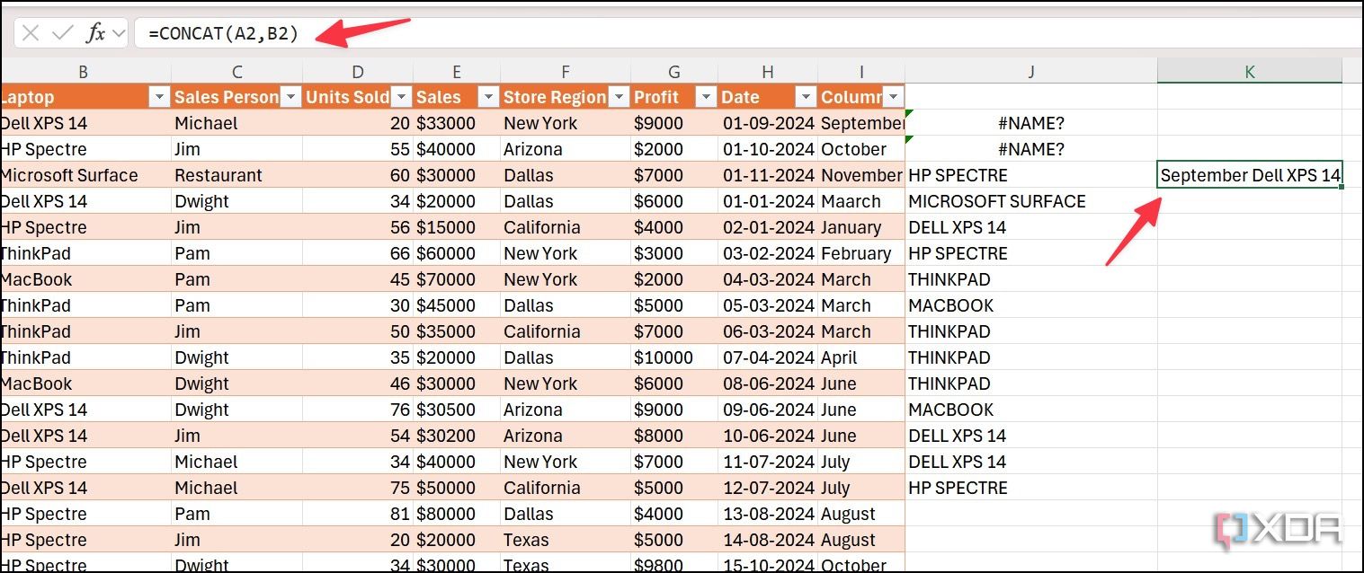
On the flip side, if you want to combine multiple text strings into one cell, use the Concatenate function.

1. Create a new column and select the first cell.
2. Type =CONCAT(cell reference). For example =CONCAT(J6,K6).
3. Press Enter and check the result. Drag and drop the cell to the bottom to apply the same on the entire column.

   

Tidy data, better results

Dealing with inconsistent data in Excel is never a good idea. By following the tricks above, you can easily master the art of data cleaning in Excel. Aside from aesthetics, it also delivers reliable insights and accurate reporting and helps in informed decision-making. Make sure to invest a little time and effort in cleaning your datasets and pave the way for more impactful results.

When it comes to data analysis, you can also use Microsoft Copilot to eliminate tedious and manual work. Check out our separate guide to power up your Excel spreadsheet with Microsoft Copilot.