Here is how I created a holiday budget planner in Excel that actually works

Holidays are typically associated with joy, family gatherings, travel, and the creation of lasting memories. However, they can also present financial challenges, especially when you are not into budgeting but should be. Overspending is a common concern, leaving many with a post-holiday debt hangover. If you want to take control of your holiday spending, this budget planner is right for you.

While there is no shortage of budgeting apps, nothing beats a fully customized spreadsheet tailored to your holiday priorities. It breaks down every category, from travel and accommodation to gifts for loved ones. By setting clear spending limits, you can enjoy the festivities without the financial guilt trip later.

Create a new Excel sheet

Microsoft Excel boasts a rich template library. But here’s the thing: relying solely on these generic templates can be like squeezing yourself into a one-size-fits-all outfit. It kind of works, but it’s not a perfect fit all the time. Crafting a custom Excel sheet often trumps using a template, especially when you want something as personalized as a holiday budget.

Besides, these templates often come with pre-set formulas and layouts that can be restrictive. Creating a custom sheet removes such hurdles and gives you a fantastic opportunity to level up your Excel game. You can learn new formulas, formatting tricks, and data organization skills. That’s why I will start with a new Excel sheet here, for your inspiration.

1. Open Microsoft Excel and create a blank workbook.
2. Enter a large header at the top and add a shade of your choice.
3. You can resize columns and rows based on your preferences. After all, you shouldn’t compromise on esthetics for your holiday budget planner.

   

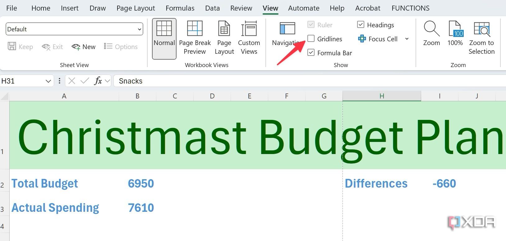
You can also hide the gridlines from your Excel workbook to simplify the look. It’s optional, though. I prefer to keep such workbooks free of lines. If you are among them, use the steps below.

1. Head to the View tab and expand Show.
2. Disable the checkmark beside Gridlines.
3. Enjoy a clean Excel look without any lines.

   

Now, we have set the stage to add relevant databases next.

Related

15 best Excel plugins that you need to be using

Must-have Excel add-ins you can’t afford to ignore

Insert relevant categories

Once the basics are set in your Excel workbook, it’s time to add expense categories that you are anticipating during holidays. For myself, I have added Gifts, Travel, Entertainment, and Holiday Meals. You can customize it the way you want and even add new ones.

1. Open your Excel sheet and add relevant expense categories.
2. For headings, make sure to use bold formatting, increase text size, and align to the middle for a better look.
3. In the example below, I have added two categories at the top and two at the bottom.

   

As always, you can change column and row size to make them prominent and easily identifiable in the workbook.

Add items and budget details

Now that your holiday budget databases are set, add items and set a budget for each one of them. Let’s take Gifts, for example.

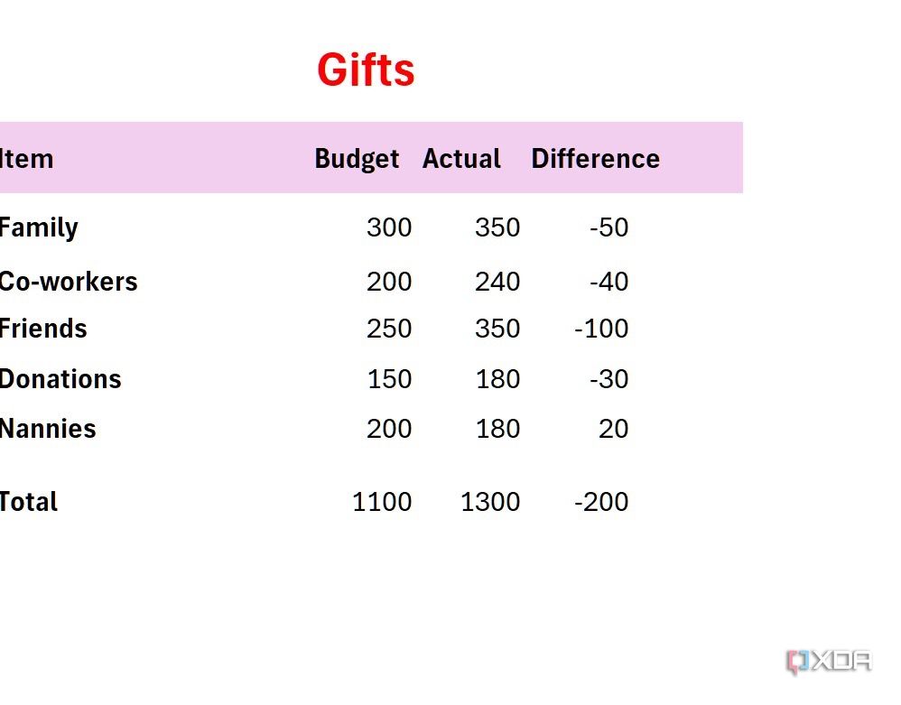
1. Under the Gift database, I have added details like Family, Co-workers, Friends, Donations, and Nannies then set a budget for each of them.

   

2. You can always get creative and include additional columns like gift products, purchase sources (Amazon, Walmart, eBay, etc.), and even dates to keep track of them. The possibilities are endless with Excel.
3. Write down the budget you wish to set for them, and once your shopping is over, enter the actual value as well.
4. Create a Total row at the bottom where you can use the AutoSum formula to calculate overall spending on gifts. It’s quite simple. Select all the cells in the Budget column, head to Formulas at the top, and select AutoSum. Do the same for Actual numbers as well.

   

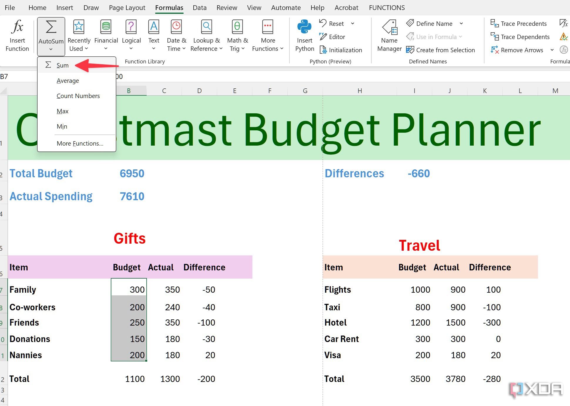
5. In the Differences column, select the first cell, then type =(B7-C7) or the cells where your first budget and actual value numbers live. Here, I have calculated the differences between the allocated budget and actual spending.

   

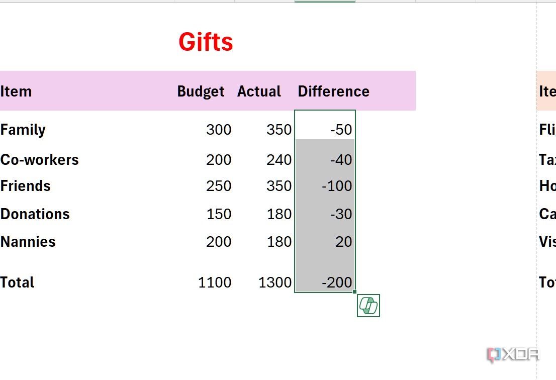
6. Once you have the first formula working, select it and drag it down to the bottom of this section to calculate the differences automatically.

Now, repeat the same for all the other databases. And remember, you can always add more columns for your convenience.

Use conditional formatting

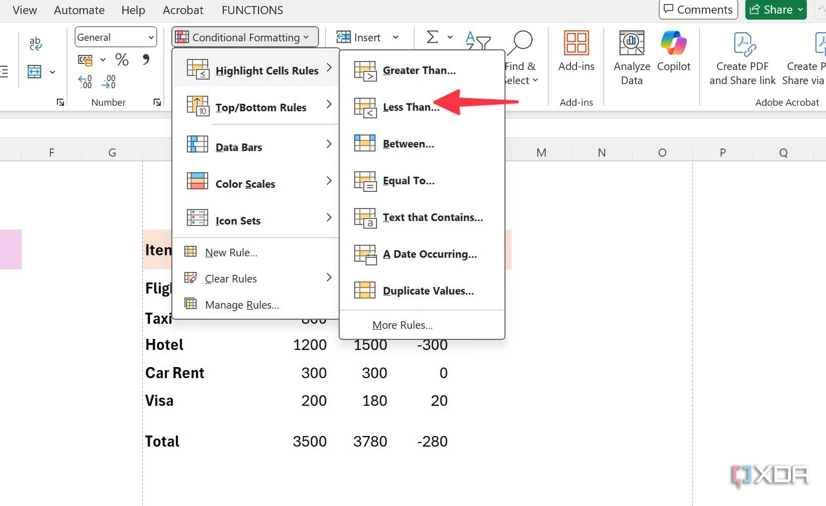
Once your database is ready, explore conditional formatting to highlight cells where the difference is in the negatives (less than 0). Basically, it points out the cells where you have spent more than the allocated budget. Instead of doing it manually, you can use conditional formatting by following the steps below.

1. Select all the cells in your Excel workbook. Head to the Home tab and select Conditional Formatting.
2. Expand Highlight Cells Rules and select Less than.

   

3. Write 0 under Format cells that are less than. Pick one of the formatting options or select Custom Format. You can pick specific fill color, fonts, border, and more. Select OK and you are good to go.

   

   

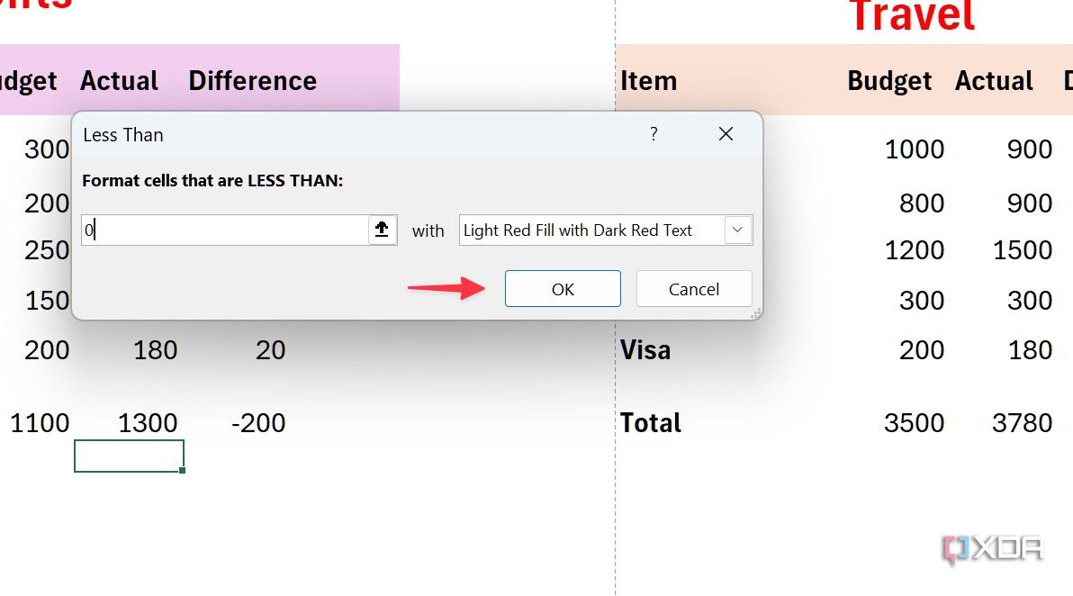
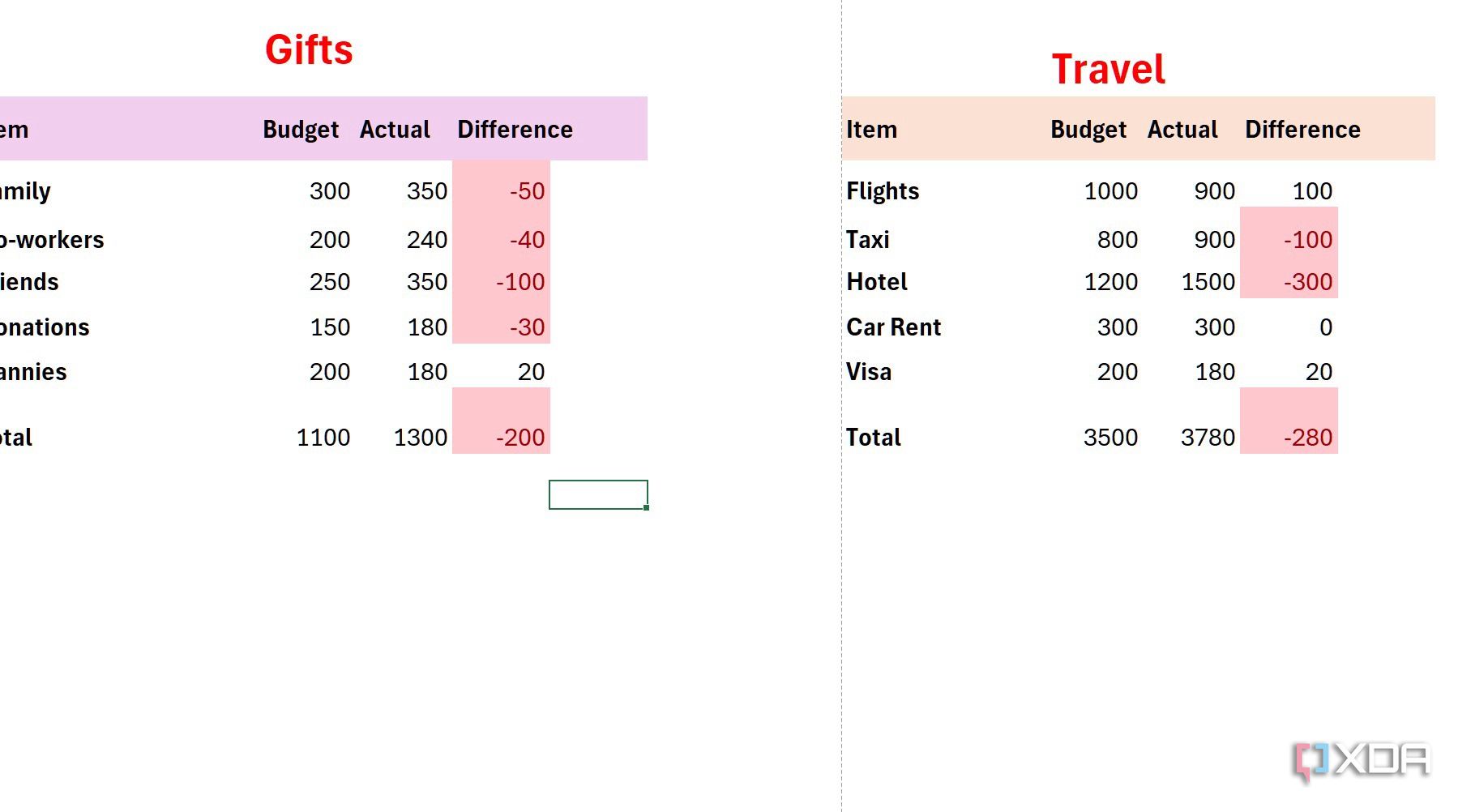
Excel should automatically highlight such cells for better understanding.

Related

12 Excel functions everyone should know about

Essential Microsoft Excel functions to streamline your everyday tasks

Explore different charts to analyze data

If you prefer some visualization, explore the built-in charts. Let’s take the Gifts table, for example.

1. Open your Excel workbook and select the entire Gift database.
2. Head to Insert at the top and expand Charts.

   

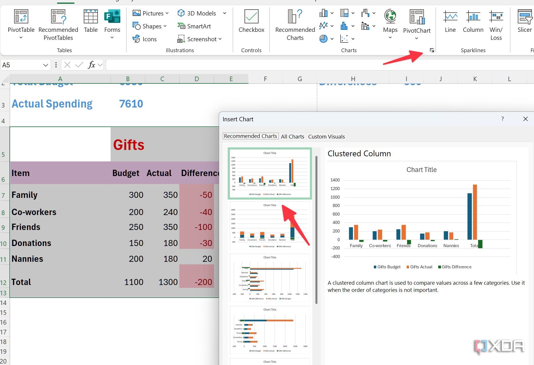
3. Pick one of the charts from the recommendations and insert it in your Excel workbook.
4. As always, you can customize the chart with different styles, colors, text positions, and more.

   

These charts do come in handy when you deal with a large database and want to glance over the spending pattern quickly.

Related

How to analyze data in Excel like a pro with pivot tables

Explore pivot tables to transform from a beginner to an analyst in minutes

Calculate the overall budget

Now, it’s time to calculate and add the overall budget summary at the top. You can add two cells, Total Budget and Actual Spending, and follow the steps below.

1. Use the SUM formula and calculate the total budget which in my case is =SUM(B12,I12,B34,I34), but you can fill in the cell values that correspond to each category’s total budget amount.
2. Use the same formula to calculate total actual spending with the same method.

   

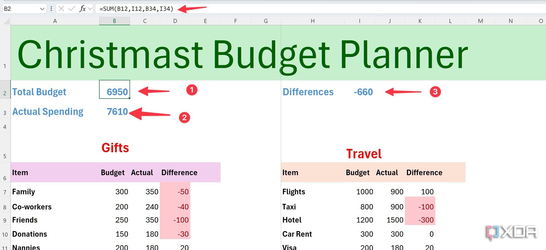
3. If you’d like to calculate the overall difference, you can use subtraction such as =B2-B3 to view the outcome.

Taming the holiday spending beast

My holiday budget planner is designed to keep the festive season merry and bright without any financial stress. Plan ahead, break down your expenses, set realistic limits, and use conditional formatting and charts to analyze the data.

Remember, this is just a sample spreadsheet. You can create a custom one based on your needs and priorities. If you prefer not to create a spreadsheet from scratch, consider using these top Excel templates to save some time.