How I built a budgeting template from scratch in Excel

When it comes to budgeting and personal finance, there is no one-size-fits-all solution. While there is no shortage of expense management apps out there, none of them quite suit my needs. This is why I decided to take matters into my own hands and have created a budgeting template in Excel. It was easier than I thought, and now I can reuse this template and remain in complete control of my finances.

In this post, I’ll break down exactly how I did it, step-by-step, so you can create your own Excel budgeting masterpiece that reflects your financial goals and habits.

Start with a blank Excel workbook

In the example below, I will create a monthly budget book with expenses, categories, allocated funds, and actual expenses, then calculate the difference between them to get a better idea. I will also show you how to use pivot tables and charts to analyze the data better and explore conditional formatting to point out specific cells automatically. Without further ado, let’s get started.

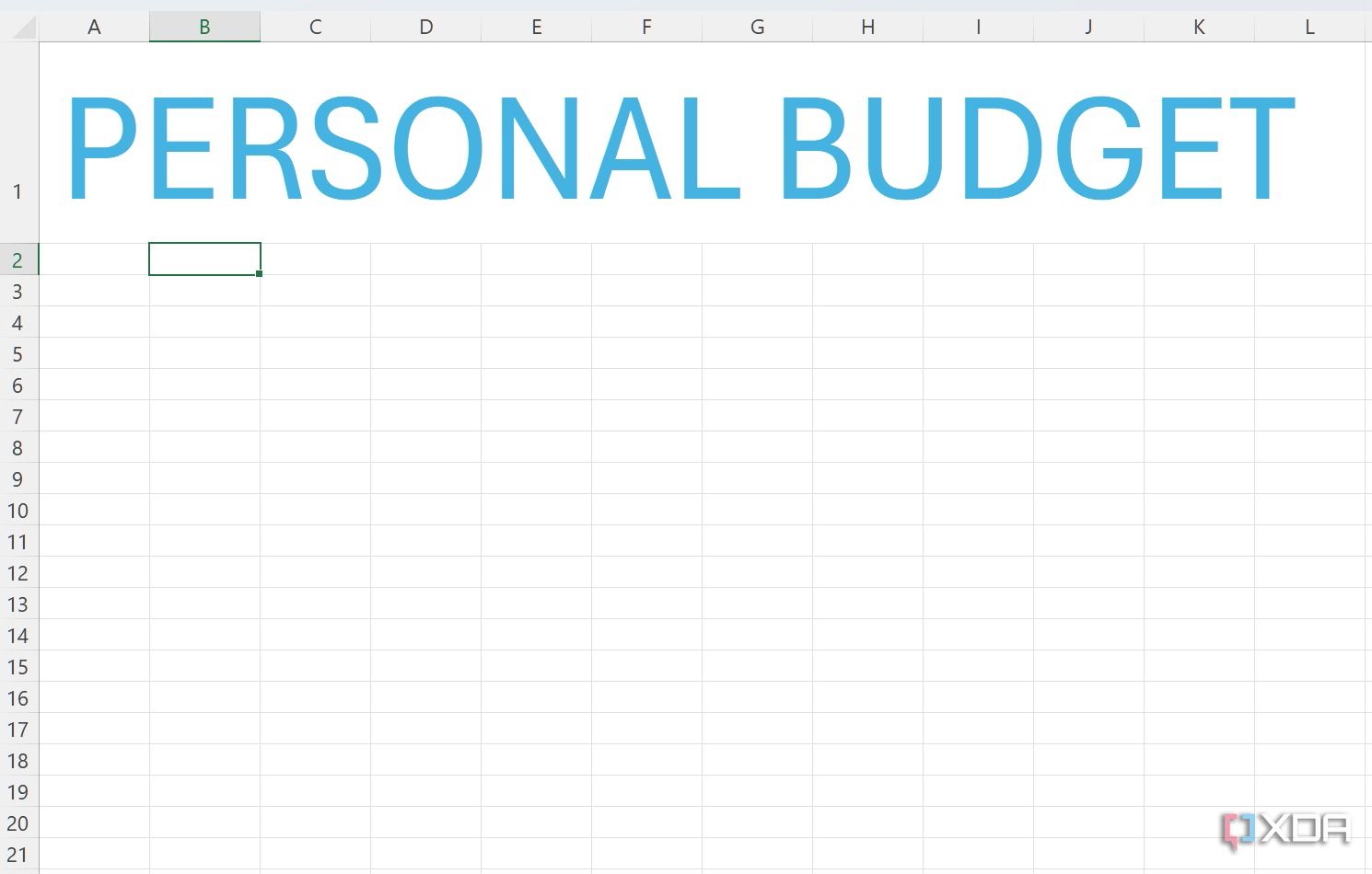
1. Open Excel and select Blank workbook.
2. Give it a nice Personal Budget header at the top to set the tone.

   

Insert columns and create a table

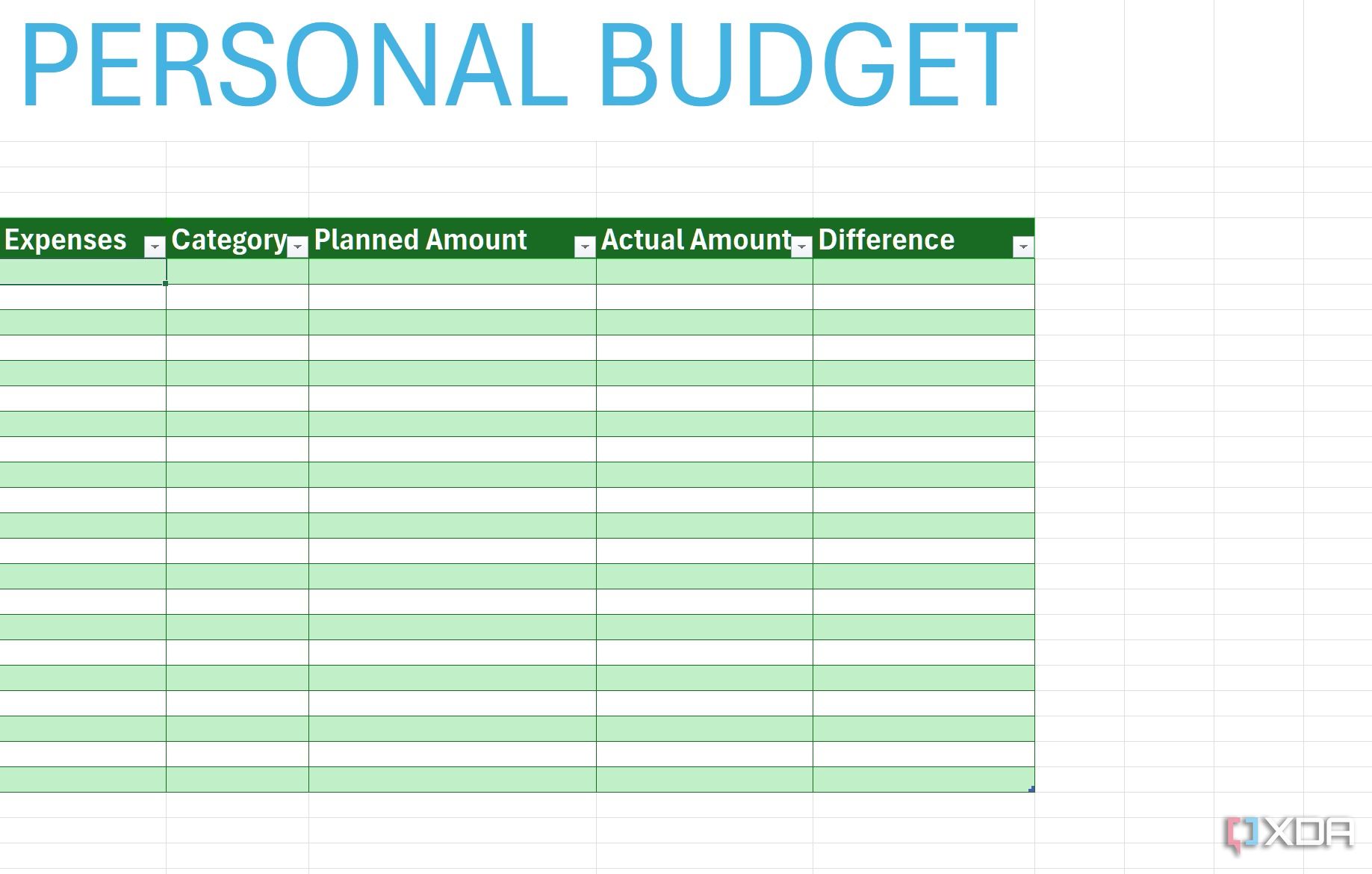
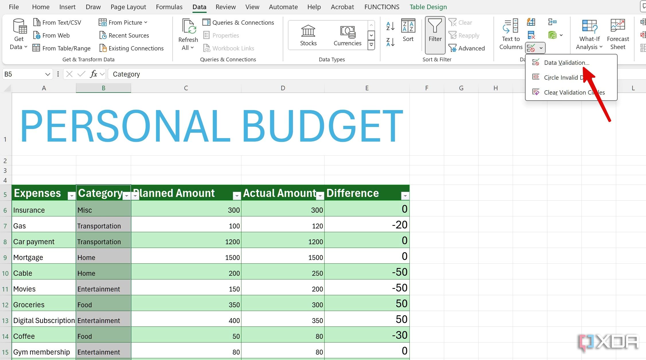
Now, we will insert relevant columns and create a table from them. In the screenshot below, I have added multiple columns like Expenses, Category, Planned Amount, Actual Amount, and Difference.

Now, let’s convert the database into a table.

1. Select your database and select Format as Table at the top.

   

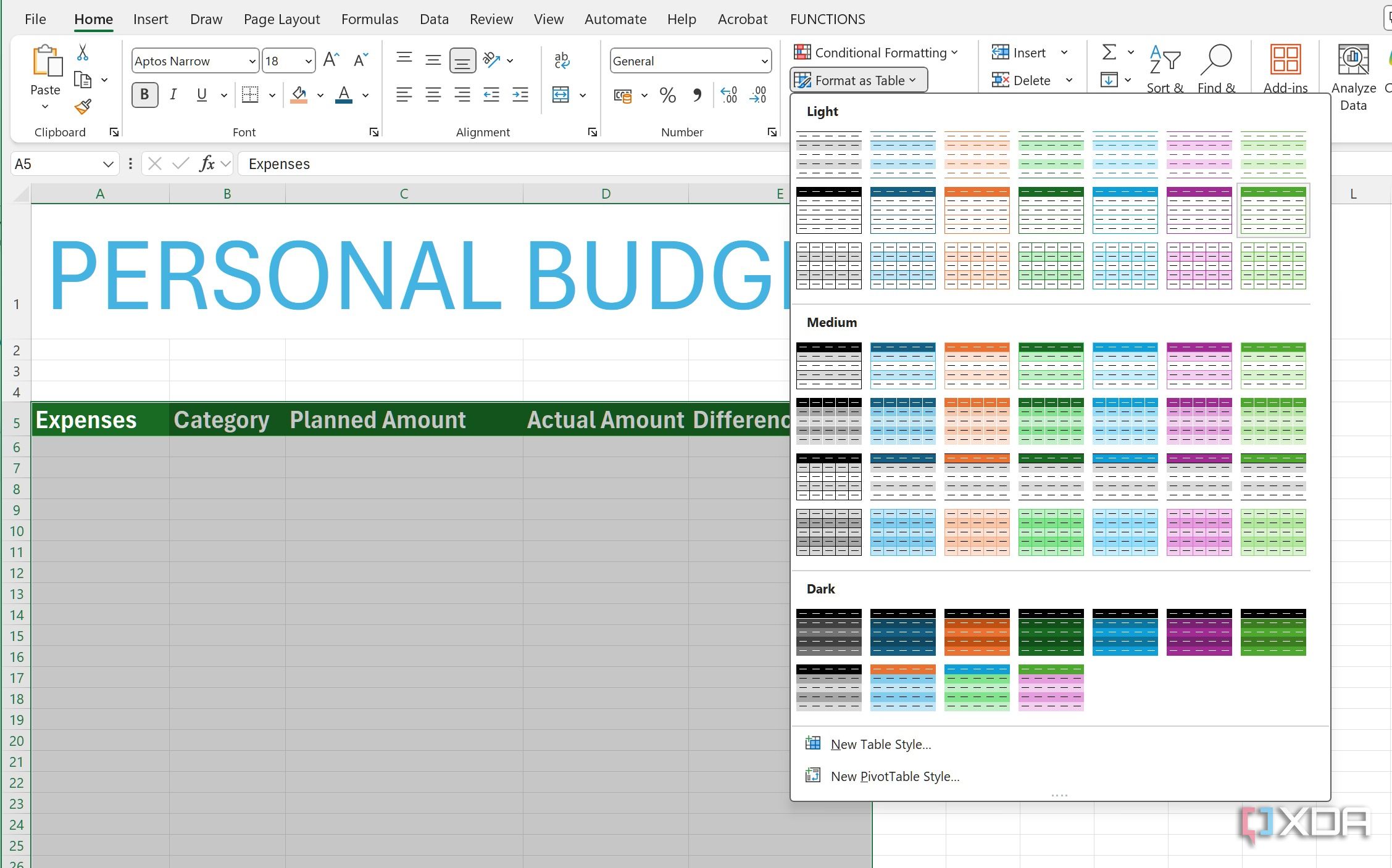
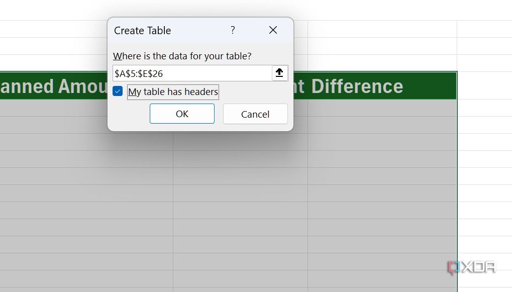
2. Pick a relevant style, click the check mark beside My table has headers and click OK.

   

3. Your table is ready to use.

   

Add budget categories

You will surely want to insert the relevant categories for all of your transactions. Let’s use data validation to enable the drop-down menu of options within the Category column. Follow the steps below.

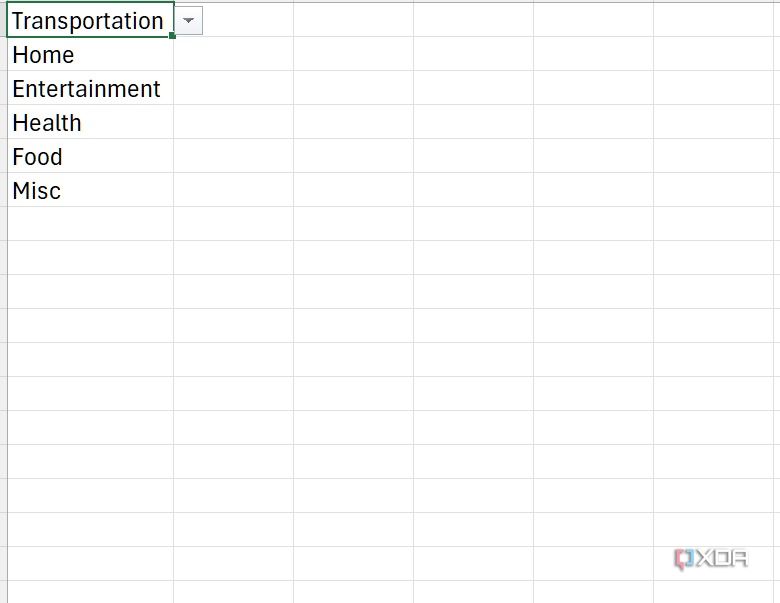
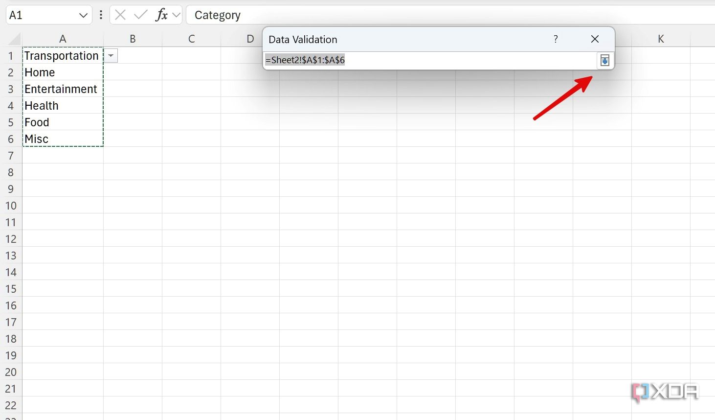
1. Create a new Excel sheet in the current workbook and write down your categories like Transportation, Home, Entertainment, Health, Food, and Misc. You can always insert more categories depending on your preferences.

   

2. Select the Category column and click Data at the top.
3. Expand Data tools and select Data Validation.

   

4. Expand Allow and select List. Click on the up arrow icon beside Source.

   

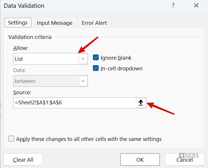
5. Select the categories which you’ve added in the other sheet, then click the down arrow.

   

6. That’s it. You can now see a drop-down menu appearing under the Category.

   

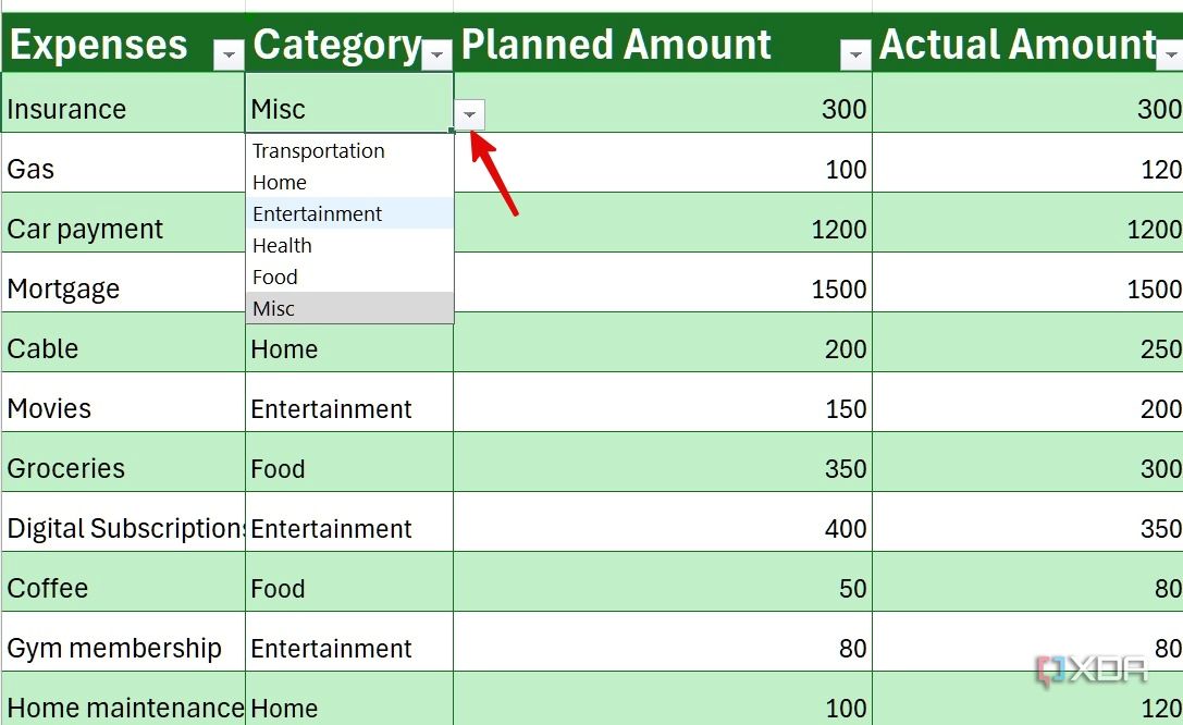
Now, assigning categories to your transactions will be much easier and faster.

Add the budget amount and calculate the difference

The basics are all set now. It’s time to create entries in your Excel workbook. You can add expenses, categories, planned and actual expenses, and more. Go through the steps below.

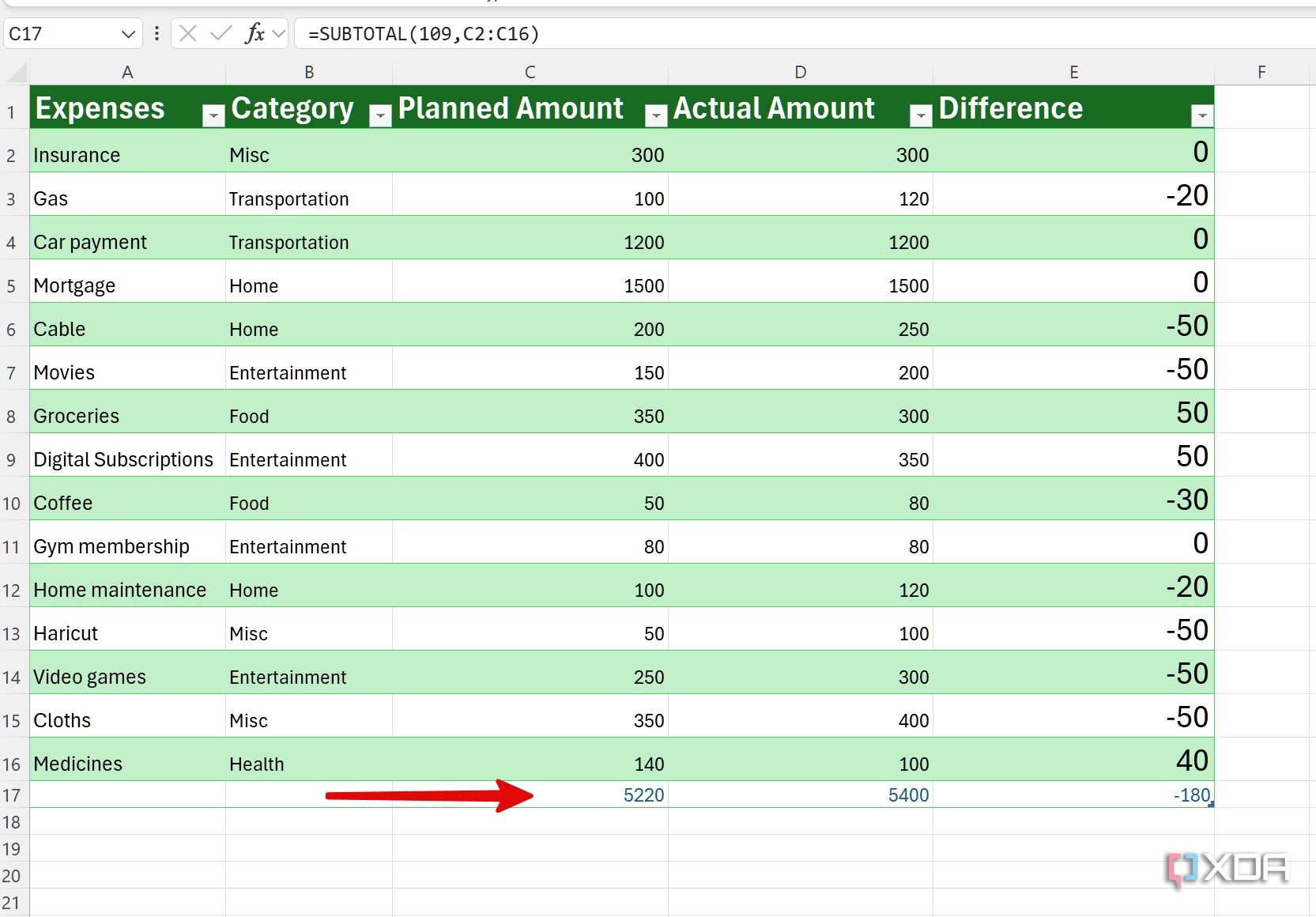
1. Add relevant expenses, use categories, and add planned and actual amounts under the columns.
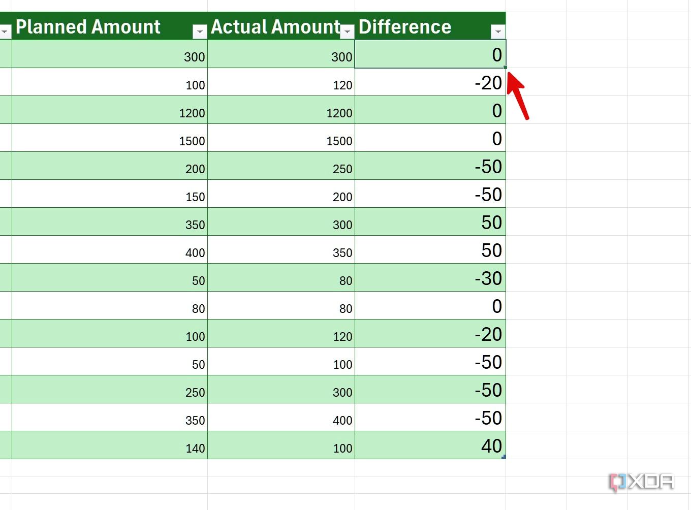
2. Move to the Difference column and select the first cell. Type =C6-D6 to calculate the difference between planned and actual amounts.

   

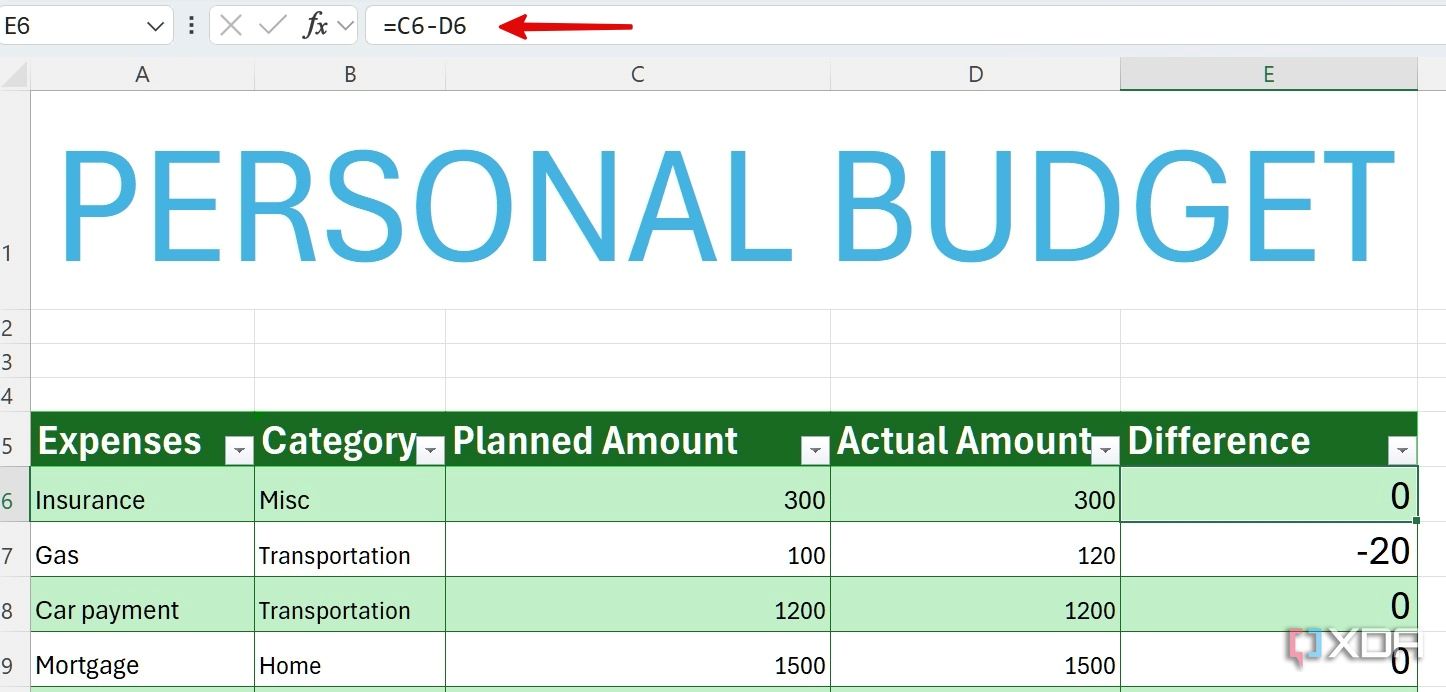
3. Move the cursor in the bottom right corner of the cell and drag it down to the end of the table to calculate the same way for all expenses.

   

4. You can calculate the total amount under the planned amount, the actual amount, and the difference at the bottom.

   

Related

How I built a to-do list in Excel that actually works

Create a functional task list in Excel for getting things done

Analyze data using pivot tables

Our ideal budget database is ready. You can now explore pivot tables and different charts to analyze the information. In the example below, I want to calculate how much I have spent on a specific category in a given month. I will calculate and use the pie chart to visualize the same using pivot tables. Go over the steps below.

1. Select your budget table and click Insert at the top.
2. Head to Tables > PivotTable > From Table/Range.

   

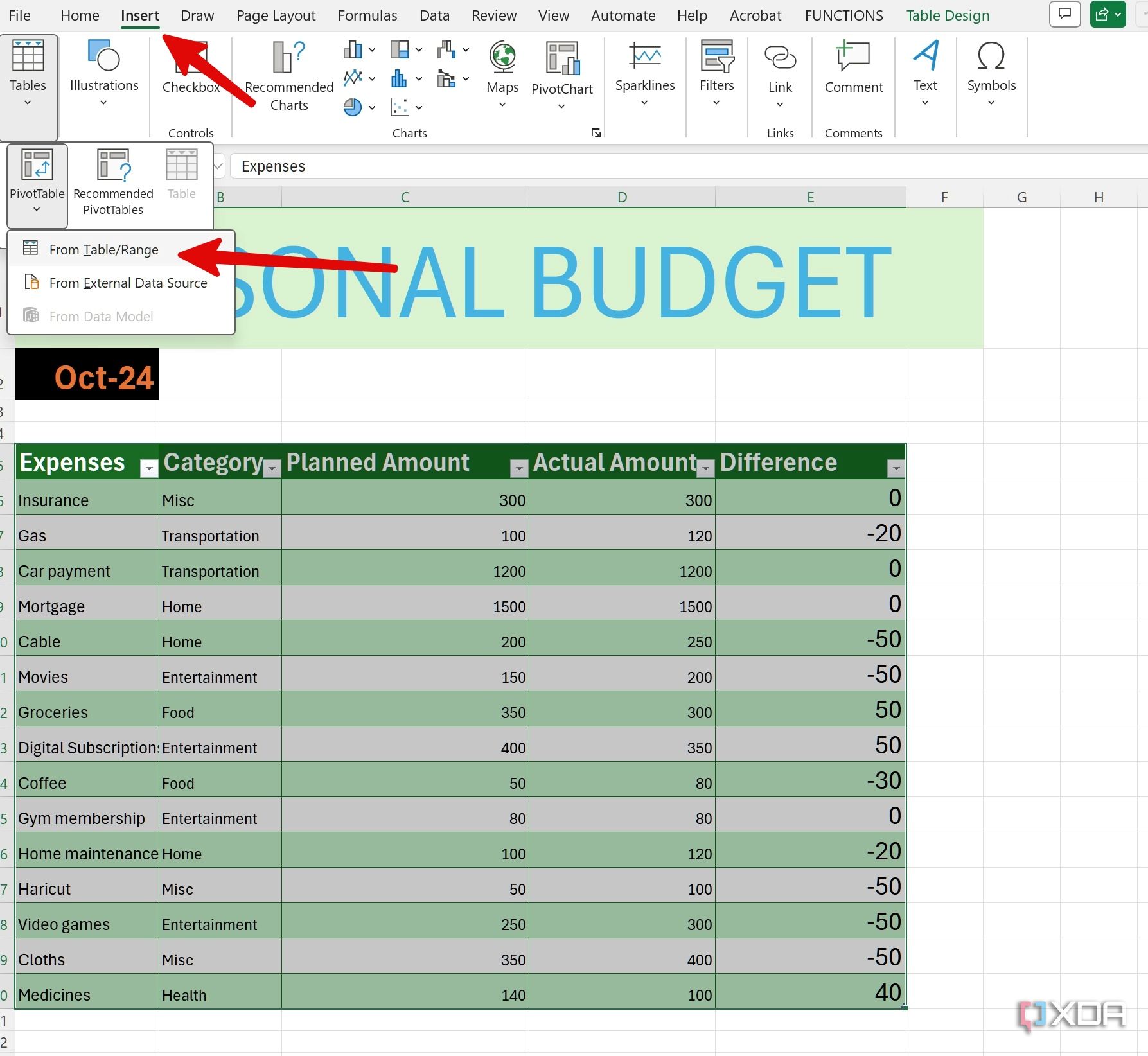
3. Click the radio button beside New Worksheet and click OK.
4. Check the PivotTable Fields from the sidebar. Click the check mark beside the elements you wish to analyze, such as Expenses, Category, and Actual Amount.

   

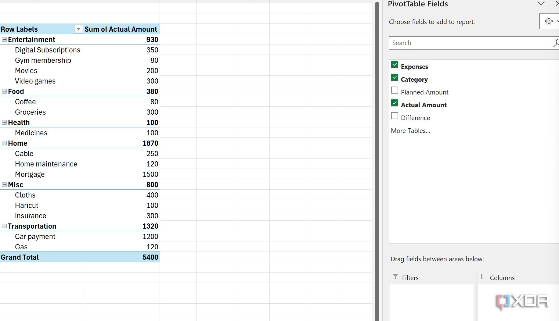
5. Glance over a custom pivot table on your sheet.
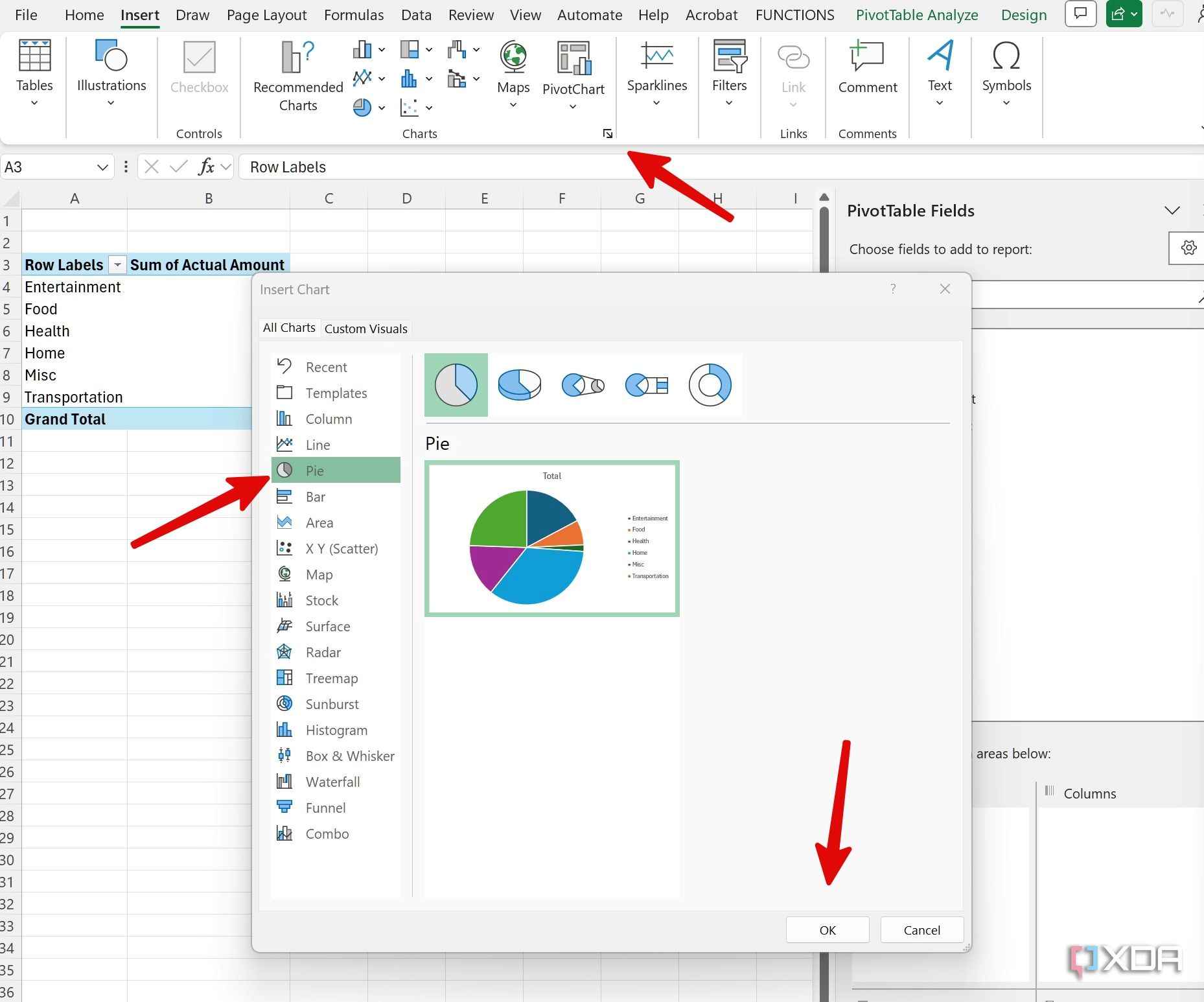
6. Open Charts under the Insert menu.
7. Select Pie and click OK to insert it.

   

8. You can click + to expand chart elements, disable chart titles, tweak data legends, and more. You can also change the chart look using the brush menu.

   

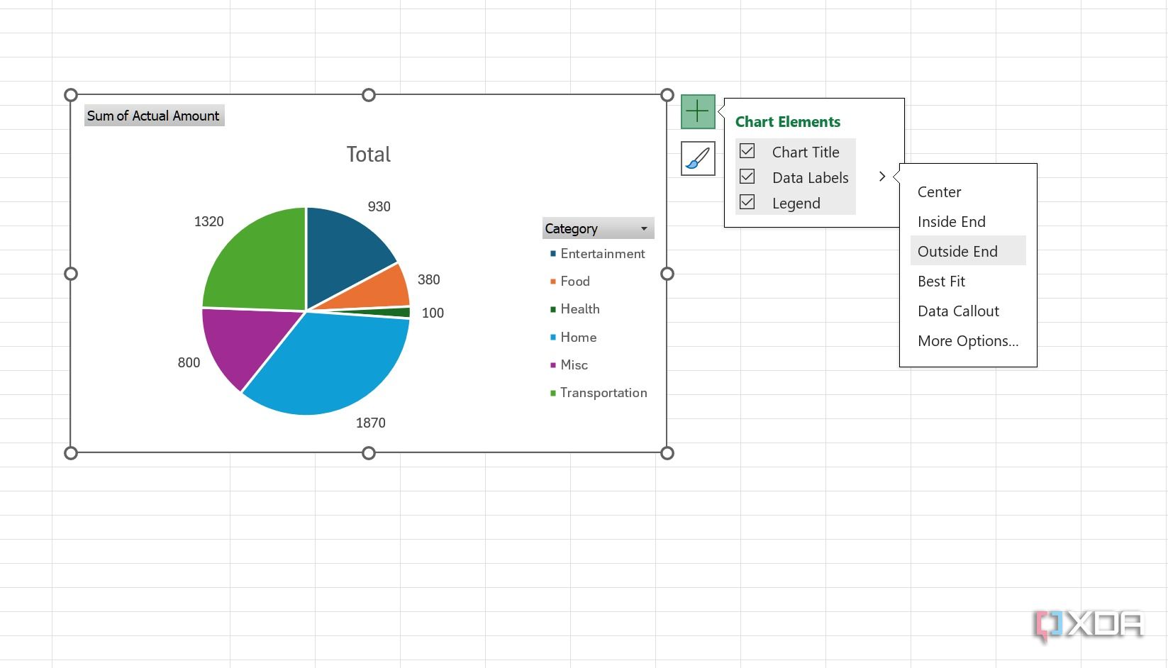
9. Copy and paste the chart to your main sheet.

   

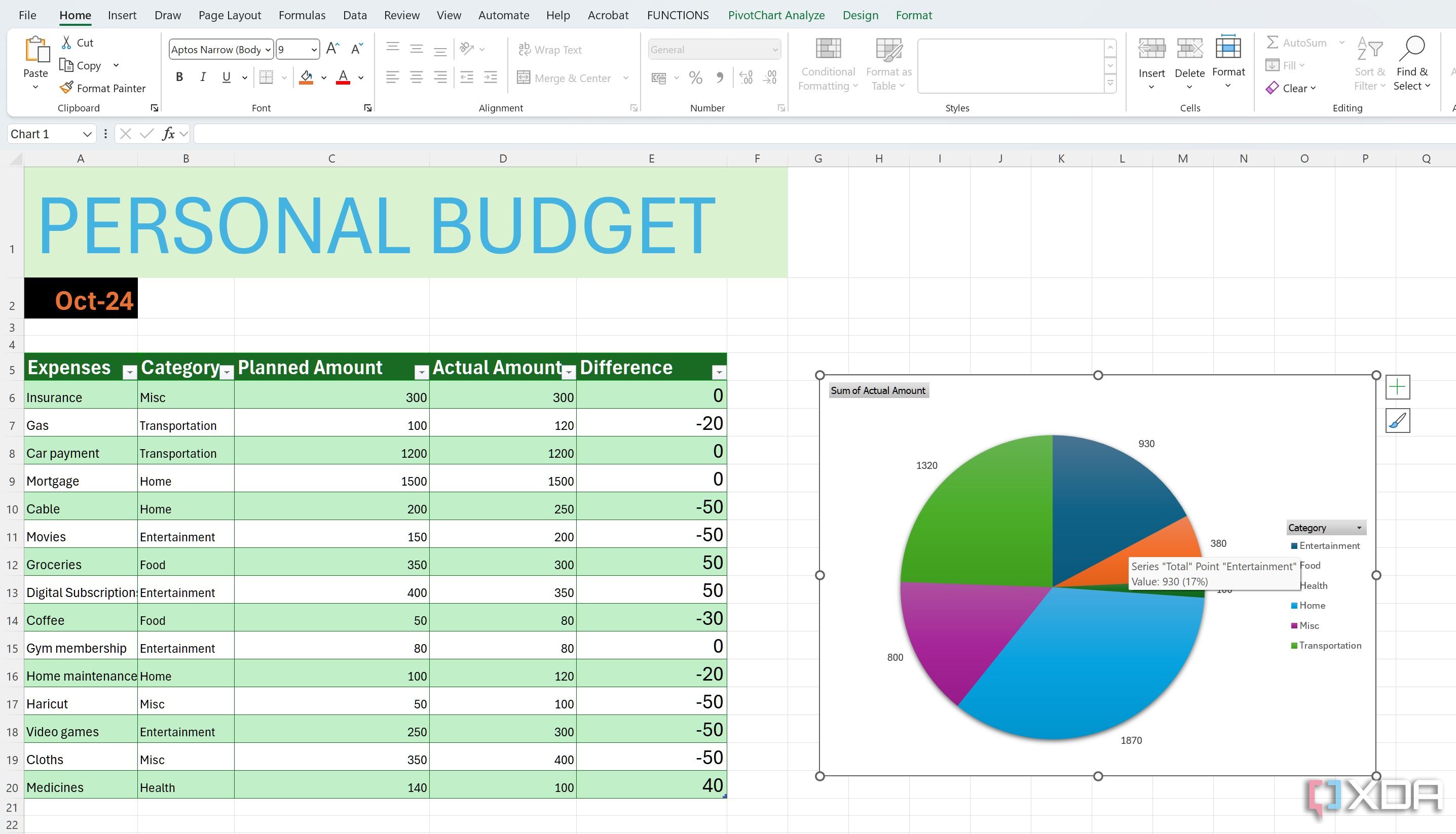
Pivot tables open up a host of possibilities to analyze your data in great depth, and can address the questions that are meaningful to you.

Related

10 free time-saver Excel templates for busy professionals

Level up your Excel game with these pro templates

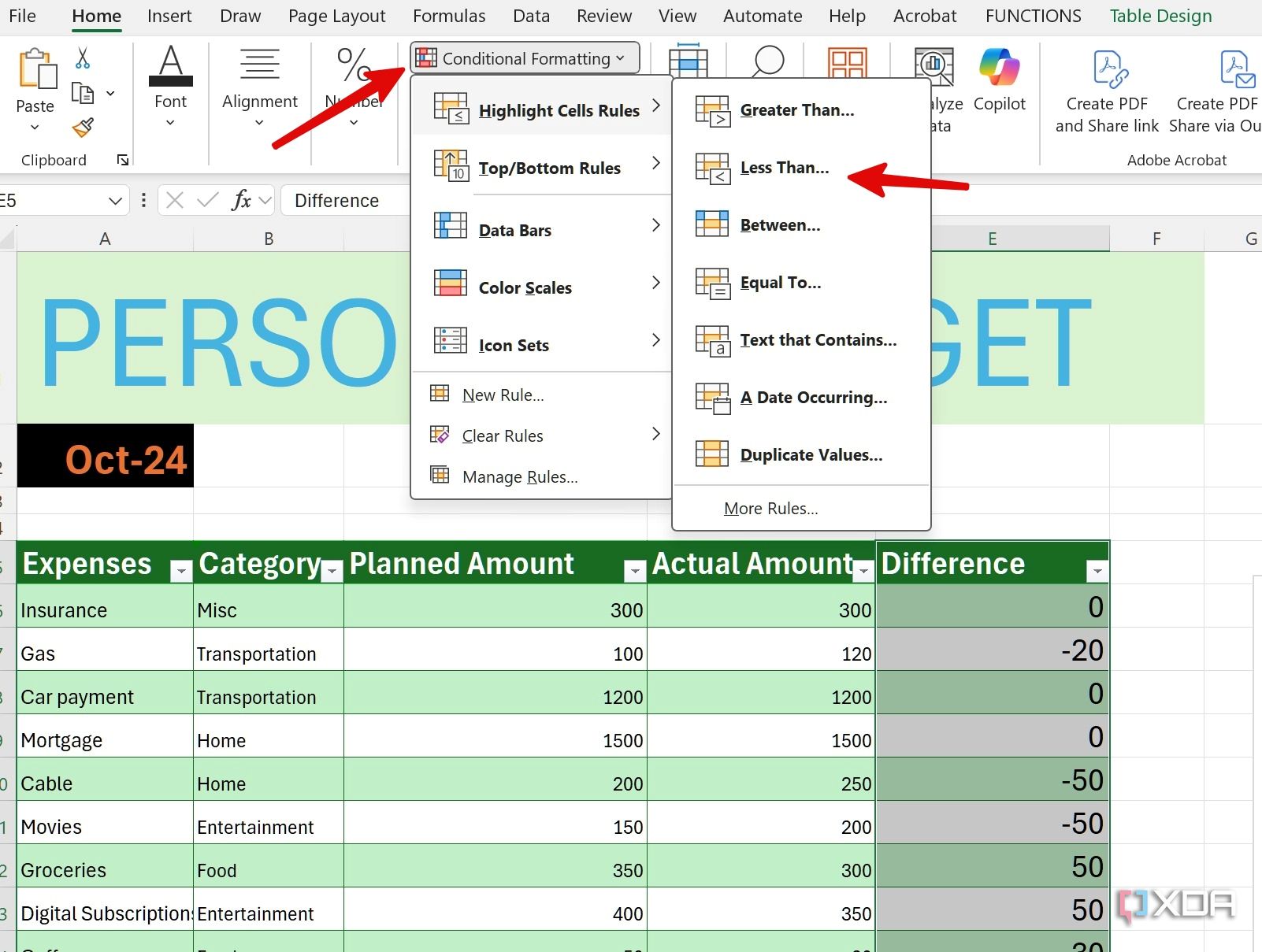
Use conditional formatting

If you want to make your budget database more dynamic and illustrative, explore conditional formatting. For instance, you could automatically highlight the cells in red when your actual expenses surpassed the planned amount. Here’s how.

1. Select Differences column and open Conditional Formatting > Highlight Cells Rules > Less Than.

   

2. Type 0 under Format cells that are LESS THAN.
3. Pick one of the format styles or select Custom format.
4. Let’s select Light Red Fill with Dark Red Text. Click Ok.

   

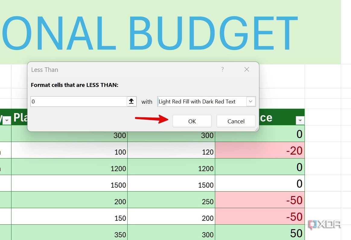
5. Excel automatically highlights such cells. Check out the screenshot below.

   

Conditional formatting offers limitless possibilities. You have the freedom to establish new rules as you see fit.

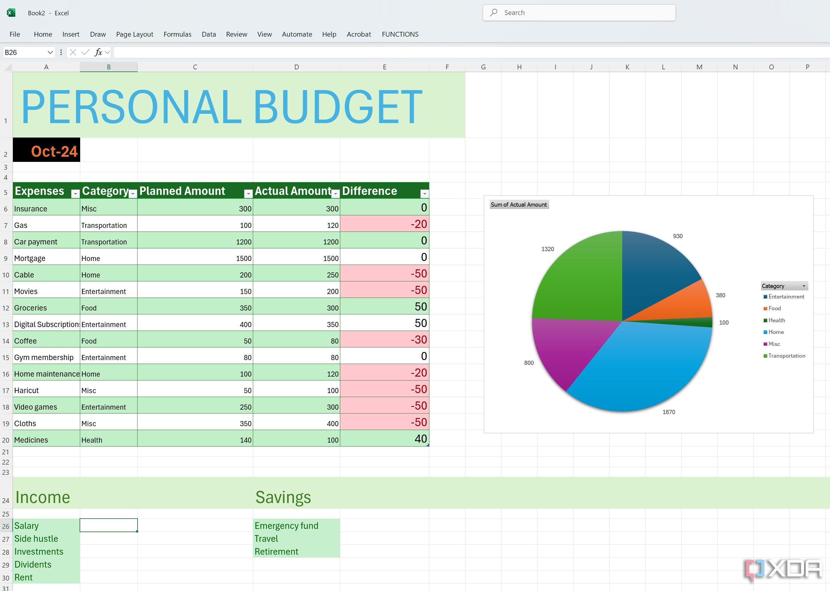
Optional: Add income and savings section

You can also add income and savings sections at the bottom to track everything in a single workbook.

You can create an Income header at the bottom (or on another sheet) and list all income sources like salary, side hustles, investments, dividends, rent, etc. Now, use the SUM function to calculate the overall income for the given month.

Similarly, create another header called Savings and list categories like emergency fund, travel, retirement, and more.

Related

15 best Excel plugins that you need to be using

Must-have Excel add-ins you can’t afford to ignore

Explore Excel budget templates

As you can see from the examples above, creating a new budgeting workbook from scratch can be time-consuming and get as involved as you want it to be. Here is where Excel templates come into play. You can head to Microsoft Create on the web and search for budget templates for Excel, to take a shortcut to your goal.

Excel-lent budgeting

Creating your own budgeting template in Excel might seem like a daunting task at first, but with a little patience and creativity, it’s totally achievable (and satisfying). What are you waiting for? Follow the steps above, create a personalized template that evolves with your needs, and gain a deeper understanding of your financial flow.

Once you start adding your expenses and income sources in Excel, your workbook will soon be filled up with hundreds of entries. Here is where you can use pivot tables to analyze your spending habits like a pro.